Flake Detection for TestGrid

In the continuous integration (CI) project workflow, developers frequently integrate code into a shared repository. Each integration can then be verified by an automated build and tests. Whenever a failure occurs in a test, developers need to manually analyze failures. Failures in the build can be legitimate or due to some other issues like an infrastructure flake, install flake, flaky test, or some other type of failure. SME’s can analyze the TestGrid data manually and determine if failures appear to be legitimate or not. However, it takes a lot of human effort and reduces the productivity of a team. In this notebook we will try to reliably detect one of these failure types: Flaky test.

What is a flaky test?

A flaky test is one that passes or fails in a nondeterministic way. See this paper for more details.

In data science terms, if a test passes and fails in an apparently random sequence then it is likely to be a flake. Tests can also be considered flaky if they pass and fail in a non-random but inconsistent pattern. Therefore, our goal here is to develop a technique for finding apparently random or inconsistent pass/fail sequences, which we can then apply to the TestGrid dataset.

import requests
import pandas as pd
import numpy as np

import matplotlib.pyplot as plt
from matplotlib import colors
import seaborn as sns
import warnings

import gzip
import json

from ipynb.fs.defs.failure_type_functions import (
    naive_flake_calc,
    calc_flakiness_score,
    calc_optimal_flakiness_score,
    flake_annotation,
    decode_run_length,
)

sns.set()
warnings.filterwarnings("ignore")

Data Access

In depth details for data access and preprocessing can be found in the testgrid_EDA notebook.

Here we provide two data access methods: download the latest or use example data. If you would like to download the most recent data for a specific grid, then please set download_data to True on line #2 below and update dashboard_name and job_name appropriately. Be warned, the output and results will likely change if the most recent data is used instead of the fixed example data.

Otherwise, we will use the repo’s example dataset data/raw/testgrid_810.json.gz

Regardless of the method used, we will be looking at “redhat-openshift-ocp-release-4.6-informing/periodic-ci-openshift-release-master-ocp-4.6-e2e-aws-proxy” as our example throughout.

## Do you want to use download data or stored data?
download_data = False

dashboard_name = "redhat-openshift-ocp-release-4.6-informing"
job_name = "periodic-ci-openshift-release-master-ocp-4.6-e2e-aws-proxy"

if download_data:
    payload = {"show-stale-tests": job_name, "tab": job_name}
    response = requests.get(
        "https://testgrid.k8s.io/" + dashboard_name + "/table", params=payload
    )
    details = pd.DataFrame(response.json()["tests"]).drop(
        [
            "linked_bugs",
            "messages",
            "user_property",
            "target",
            "original-name",
        ],
        axis=1,
    )
else:
    with gzip.open("../../data/raw/testgrid_810.json.gz", "rb") as read_file:
        data = json.load(read_file)
    details = data['"' + dashboard_name + '"'][job_name]["grid"]
    details = pd.DataFrame(details)

details.head(10)

	name	statuses
0	Overall	[{'count': 21, 'value': 12}, {'count': 1, 'val...
1	operator.Run multi-stage test e2e-aws-proxy - ...	[{'count': 9, 'value': 12}, {'count': 1, 'valu...
2	operator.Run multi-stage test e2e-aws-proxy - ...	[{'count': 9, 'value': 12}, {'count': 1, 'valu...
3	operator.Run multi-stage test e2e-aws-proxy - ...	[{'count': 9, 'value': 12}, {'count': 1, 'valu...
4	operator.Run multi-stage test e2e-aws-proxy - ...	[{'count': 9, 'value': 12}, {'count': 1, 'valu...
5	operator.Run multi-stage test e2e-aws-proxy - ...	[{'count': 9, 'value': 1}, {'count': 1, 'value...
6	[sig-api-machinery][Feature:APIServer][Late] k...	[{'count': 20, 'value': 0}, {'count': 1, 'valu...
7	[sig-auth][Feature:SCC][Early] should not have...	[{'count': 20, 'value': 0}, {'count': 1, 'valu...
8	[sig-arch] Monitor cluster while tests execute	[{'count': 20, 'value': 0}, {'count': 20, 'val...
9	[sig-node] pods should never transition back t...	[{'count': 20, 'value': 0}, {'count': 18, 'val...

From the column “statuses” above we can see that the time series data is run length encoded. Let’s add a decoded column so we can get the data in an easier to use array format.

# use the decode_run_length function imported from TestGrid_EDA notebook
details["values"] = details["statuses"].apply(decode_run_length)

details.head(10)

	name	statuses	values
0	Overall	[{'count': 21, 'value': 12}, {'count': 1, 'val...	[12, 12, 12, 12, 12, 12, 12, 12, 12, 12, 12, 1...
1	operator.Run multi-stage test e2e-aws-proxy - ...	[{'count': 9, 'value': 12}, {'count': 1, 'valu...	[12, 12, 12, 12, 12, 12, 12, 12, 12, 1, 12, 12...
2	operator.Run multi-stage test e2e-aws-proxy - ...	[{'count': 9, 'value': 12}, {'count': 1, 'valu...	[12, 12, 12, 12, 12, 12, 12, 12, 12, 1, 12, 12...
3	operator.Run multi-stage test e2e-aws-proxy - ...	[{'count': 9, 'value': 12}, {'count': 1, 'valu...	[12, 12, 12, 12, 12, 12, 12, 12, 12, 1, 12, 12...
4	operator.Run multi-stage test e2e-aws-proxy - ...	[{'count': 9, 'value': 12}, {'count': 1, 'valu...	[12, 12, 12, 12, 12, 12, 12, 12, 12, 0, 12, 12...
5	operator.Run multi-stage test e2e-aws-proxy - ...	[{'count': 9, 'value': 1}, {'count': 1, 'value...	[1, 1, 1, 1, 1, 1, 1, 1, 1, 0, 1, 1, 1, 1, 1, ...
6	[sig-api-machinery][Feature:APIServer][Late] k...	[{'count': 20, 'value': 0}, {'count': 1, 'valu...	[0, 0, 0, 0, 0, 0, 0, 0, 0, 0, 0, 0, 0, 0, 0, ...
7	[sig-auth][Feature:SCC][Early] should not have...	[{'count': 20, 'value': 0}, {'count': 1, 'valu...	[0, 0, 0, 0, 0, 0, 0, 0, 0, 0, 0, 0, 0, 0, 0, ...
8	[sig-arch] Monitor cluster while tests execute	[{'count': 20, 'value': 0}, {'count': 20, 'val...	[0, 0, 0, 0, 0, 0, 0, 0, 0, 0, 0, 0, 0, 0, 0, ...
9	[sig-node] pods should never transition back t...	[{'count': 20, 'value': 0}, {'count': 18, 'val...	[0, 0, 0, 0, 0, 0, 0, 0, 0, 0, 0, 0, 0, 0, 0, ...

TestGrids are made of a set of tests that either pass or fail over time. They are multidimensional time series where the values can take either 0 (not run), 1 (pass), 12 (fail), or 13(flaky).

Now that we have all our data unrolled, lets plot it. We will use green for pass (1), red for fail (12), white for not run (0) and purple for flaky (13). We will also just plot the first 40 rows to save some space.

plt.figure(figsize=(20, 10))
cmap = colors.ListedColormap(["white", "green", "red", "purple"])
norm = colors.BoundaryNorm(boundaries=[0, 1, 12, 13], ncolors=3)
sns.heatmap(
    np.array(list(details["values"].values))[:40],
    fmt="",
    cmap=cmap,
    norm=norm,
    cbar=False,
    linewidths=0.1,
    linecolor="Black",
)
plt.ylabel("Tests")
plt.xlabel("Days")
plt.title(
    "Redhat-openshift-ocp-release-4.6-informing/periodic-ci-\
openshift-release-master-ocp-4.6-e2e-aws-proxy\n",
    fontsize=20,
)
plt.show()

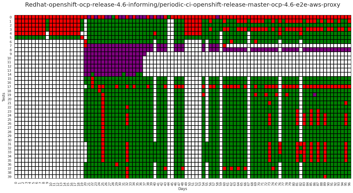
Cells with Purple color in the above graph are the existing flake labels defined by the build process. Currently, each failed test is retried, and if it passes on a subsequent run it is considered to be flaky.

We can see from the grid above that there is a large chunk of flakes between test 7 and 15, but there is also a fair amount of irregular pass/failure patterns on the grid that are not being flagged. Let’s see if we can create a method to better capture these flakes.

Flaky test detection

In the following section, we will explore different methods to detect flaky tests.

Naive flakiness method

This method calculates flakiness as a ratio of failed or flaky tests to total tests. The idea being that a score of 50 would mean a 50/50 (random) chance of a pass or fail occurring, indicating a flaky test. The major drawback of this method is that it evaluates the time series as a whole and can’t account for specific pass/fail patterns or sub-sequences. If the first half of a series are all pass and the second half are all fail, we would not consider that to be a flake, despite this method flagging it as such.

This is all to say, this is our naive baseline we can use to ensure our later methods are performing well.

test_array = [1] * 6 + [12] * 11 + [1] * 7
plt.figure(figsize=(20, 5))
plt.plot(test_array)
plt.title("Consecutive Failures", fontsize=20)
plt.xlabel("time")
plt.show()
print(f"Naive Flake Score {naive_flake_calc(test_array)}")

Naive Flake Score 45.833333333333336

In the above cell, we have shown a drawback of the naive flakiness method. As we can see, we have a test array that consist of consecutive test failures, which is not an attribute of a flaky test. However, we got a very high flakiness score.

Flip flakiness method

As we discussed earlier, flaky tests pass and fail across multiple runs over a certain period of time. We can characterize this behavior by using the concept of an edge. Here we will define an edge as the transition of a particular test case from pass to fail (or fail to pass). Let’s look at a couple examples below to illustrate the idea further.

plt.figure(figsize=(20, 10))  # instantiating figure to be 5"x5", 100 dpi resolution


test_array = [1] * 6 + [12] * 11 + [1] * 7
x = np.arange(len(test_array))
plt.subplot(2, 1, 1, aspect=0.3)
plt.step(x, test_array)
plt.title("Single edge and multiple fails", fontsize=20)

plt.subplot(2, 1, 2, aspect=0.3)
test_array_1 = [1] * 5 + [1, 12] * 8 + [1] * 3
plt.step(x, test_array_1)
plt.title("multiple edges and multiple fails", fontsize=20)


plt.show()

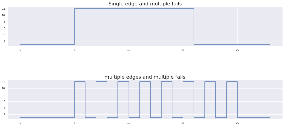
In the images above, we have shown example results for 25 test runs. In the first image we can see there are multiple fails but only a single edge. In the second image, we have fewer fails but many more edges. Therefore, the second test exhibits a more erratic behavior pattern, and one we would associate more with a flaky test.

We calculated the flakiness score as the number of edges divided by total runs. The most common approach to detect flaky test is to run flaky test multiple times and if it passes in any run then it is not considered to be a flaky test (please see paper for details). At Google, for example, if a test fails three times in a row, only then is it reported as a real failure; otherwise, it’s considered a flake please see blog for details. We will follow suite and also ignore three or more consecutive failures when calculating a flakiness score.

For the flip flakiness method below the possible scores will lie between 0 and 50; where 0 is no flakiness and 50 is maximum flakiness.

Below, we have tested our function using some basic test cases.

plt.figure(figsize=(20, 5))
x = np.arange(len(test_array))
plt.step(x, test_array)
plt.title("Single edge and multiple fails", fontsize=20)
plt.ylim(1, 13)
plt.show()
print(
    "flip-flakiness score: ",
    calc_flakiness_score(test_array),
)

flip-flakiness score:  0.0

In the above figure, we can see there is only one edge with more than three consecutive failures. Hence we did not consider the above test as a flaky test. Hence, the total flakiness score using the flip flakiness method is 0

plt.figure(figsize=(20, 5))
x = np.arange(len(test_array_1))
plt.step(x, test_array_1)
plt.ylim(1, 13)
plt.title("multiple edges and multiple fails", fontsize=20)
plt.show()

print(
    "flip-flakiness score: ",
    calc_flakiness_score(test_array_1),
)

flip-flakiness score:  33.33333333333333

In the above figure, we can see there are multiples edges. Hence, this test exhibits a more flake-like behavior pattern. Therefore, our flakiness score is greater.

plt.figure(figsize=(20, 5))
test_array_7 = [1, 12] * 11
x = np.arange(len(test_array_7))
plt.step(x, test_array_7)
plt.title("more multiple edges and multiple fails", fontsize=20)
plt.show()
print(
    "flip-flakiness score: ",
    calc_flakiness_score(test_array_7),
)

flip-flakiness score:  50.0

In the above figure, we have simulated an extremely flaky test with an inconsistent pass behavior pattern. And as you can see we get a maximum flakiness score of 50.

plt.figure(figsize=(20, 5))
test_array_2 = [1] * 24
x = np.arange(len(test_array_2))
plt.step(x, test_array_2)
plt.ylim(0, 13)
plt.title("all tests pass", fontsize=20)
plt.show()

print(
    "flip-flakiness score: ",
    calc_flakiness_score(test_array_2),
)

flip-flakiness score:  0.0

In the above figure, we can see all the test runs passed. And as we would expect, our flakiness score is 0

plt.figure(figsize=(20, 5))
test_array_3 = [12] * 24
x = np.arange(len(test_array_3))
plt.step(x, test_array_3)
plt.ylim(1, 13)
plt.title("all tests fail", fontsize=20)
plt.show()

print(
    "flip-flakiness score: ",
    calc_flakiness_score(test_array_3),
)

flip-flakiness score:  0.0

In the above example, we can see that there are no edges and consistent failures occurring for each run. We do not consider this pattern to represent a flake, so the flakiness score using the flip flakiness method is 0.

plt.figure(figsize=(20, 5))
test_array_4 = [12, 0] * 2 + [12] * 5 + [0] * 2 + [12] * 7
x = np.arange(len(test_array_4))
plt.step(x, test_array_4)
plt.ylim(0, 13)
plt.title("fail or not run tests", fontsize=20)
plt.show()

print(
    "flip-flakiness score: ",
    calc_flakiness_score(test_array_4),
)

flip-flakiness score:  0.0

In the above example we have simulated consistent failures with irregular non-run instances. As we can see, this method has ignored the not run instances in our calculation of flakiness score.

In addition to the examples above, we have also included the test cases used by the TestGrid developers below.

test_array_google_1 = []
print(
    "Empty list:",
    "Passed" if calc_flakiness_score(test_array_google_1) == 0 else "Failed",
)
test_array_google_2 = [1, 1, 1]
print(
    "All passing:",
    "Passed" if calc_flakiness_score(test_array_google_2) == 0 else "Failed",
)
test_array_google_3 = [1, 12, 1, 1, 13, 1, 1, 1, 1, 12]
print(
    "Multiple flakes:",
    "Passed" if calc_flakiness_score(test_array_google_3) == 30 else "Failed",
)
test_array_google_4 = [1, 12, 12, 1, 1, 1, 1, 12, 1, 1]
print(
    "Short run:",
    "Passed" if calc_flakiness_score(test_array_google_4) == 20 else "Failed",
)
test_array_google_5 = [1, 12, 12, 12, 12, 12, 1, 12, 1, 12]
print(
    "Long run:",
    "Passed" if calc_flakiness_score(test_array_google_5) == 40 else "Failed",
)
test_array_google_6 = [1, 12, 12, 13, 12, 12, 1, 12, 1, 12]
print(
    "Long run interupted by flakes:",
    "Passed" if calc_flakiness_score(test_array_google_6) == 50 else "Failed",
)

Empty list: Passed
All passing: Passed
Multiple flakes: Passed
Short run: Passed
Long run: Passed
Long run interupted by flakes: Passed

Excellent! All tests passed. From our hand-crafted examples and the tests cases above we can conclude that the flip flakiness method we have used here performs at least on par with the methods implemented by TestGrid.

One drawback of this method you may have noticed is that it evaluates the entire pass/fail time series for each test, and does not account for possible flaky subset within an otherwise stable test. Let’s extend this method to find flaky regions (subsets) in our test data.

Flip Flakiness with Optimal Distance

One of the downsides of finding a single value for each test case is that there might be two different consecutive time periods for which the test case is behaving flaky, or the number of edges is relatively low compared to total runs. This could lead to a low flakiness score, despite the test is still being flaky. Let’s illustrate this statement with an example.

plt.figure(figsize=(20, 5))
test_array_5 = [1] * 8 + [1, 12] * 2 + [1] * 23 + [1, 12, 1, 1, 12, 1, 12] + [1] * 16
x = np.arange(len(test_array_5))
plt.step(x, test_array_5)
plt.ylim(1, 14)
plt.title("two flaky regions", fontsize=20)
plt.show()

print(
    "flip-flakiness score: ",
    calc_flakiness_score(test_array_5),
)

flip-flakiness score:  8.620689655172415

As we can see in the above graph, we have two separate time periods for which behavior is flaky, between runs [8,11] and [35,41]. However, our flakiness score is rather low since the total number of runs is high in comparison.

To overcome this limitation, instead of calculating the flakiness score on the entire run we will calculate the flakiness score between edges to maximize our flakiness score for flaky subsets of the test.

Specifically, we calculate the flakiness score between the two farthest edges, which have a flakiness score greater than a user defined threshold. Currently, we use a threshold of flakiness score of 30, but this can tuned according to needs of an application.

plt.figure(figsize=(20, 5))
x = np.arange(len(test_array_5))
plt.step(x, test_array_5)
plt.ylim(1, 14)
plt.title("two flaky regions", fontsize=20)
plt.show()

modified_test_array, flake_dict = calc_optimal_flakiness_score(test_array_5)
print(
    "Flip Flakiness with Optimal Distance results: ",
)
for i in flake_dict.keys():
    print(f" flake between {i} with score of {flake_dict[i]}")

Flip Flakiness with Optimal Distance results: 
 flake between (8, 11) with score of 50.0
 flake between (35, 41) with score of 42.857142857142854

As we can see in the graph above, we have two separate time periods for which behavior is flaky, between runs [8,11] and [35,41]. Using flip flakiness with optimal distance we have a successfully identified these two flaky regions.

Comparison of different methods

Now that we have explored 3 different methods for identifying flakes in TestGrid data, lets compare them directly and make sure we move forward with the best method.

Comparison of custom test cases

Below we use our custom test cases to compare performance.

plt.figure(figsize=(20, 5))
x = np.arange(len(test_array))
plt.step(x, test_array)
plt.title("Single edge and multiple fails", fontsize=20)
plt.ylim(1, 13)
plt.show()

naive_score = naive_flake_calc(test_array)
total_error_naive = flake_annotation(test_array, naive_score, 10).count(13)
flip_score = calc_flakiness_score(test_array)
total_error_flip = flake_annotation(test_array, flip_score, 10).count(13)
modified_test_array, flake_dict = calc_optimal_flakiness_score(test_array, 30)
total_error_optimal_flip = modified_test_array.count(13)

print(
    "Naive Score: ",
    naive_score,
    " Number of Flaky Tests Detected: ",
    total_error_naive,
)
print(
    "Flip-Flakiness Score: ",
    flip_score,
    " Number of Flaky Tests Detected: ",
    total_error_flip,
)
print(
    "Flip Flakiness with Optimal Distance score: ",
    flake_dict,
    " Number of Flaky Tests Detected: ",
    total_error_optimal_flip,
)

Naive Score:  45.833333333333336  Number of Flaky Tests Detected:  11
Flip-Flakiness Score:  0.0  Number of Flaky Tests Detected:  0
Flip Flakiness with Optimal Distance score:  {}  Number of Flaky Tests Detected:  0

Given the above example, which we do not consider to be a flake, we can see that both Flip-Flakiness with optimal distance and Flip-Flakiness performed equally well, whereas the Naive method incorrectly flagged this example as flaky.

plt.figure(figsize=(20, 5))
x = np.arange(len(test_array_3))
plt.step(x, test_array_3)
plt.ylim(1, 13)
plt.title("all tests fail", fontsize=20)
plt.show()

naive_score = naive_flake_calc(test_array_3)
total_error_naive = flake_annotation(test_array_3, naive_score, 10).count(13)
flip_score = calc_flakiness_score(test_array_3)
total_error_flip = flake_annotation(test_array_3, flip_score, 10).count(13)
modified_test_array, flake_dict = calc_optimal_flakiness_score(test_array_3, 30)
total_error_optimal_flip = modified_test_array.count(13)

print(
    "Naive Score: ",
    naive_score,
    " Number of Flaky Tests Detected: ",
    total_error_naive,
)
print(
    "Flip-Flakiness Score: ",
    flip_score,
    " Number of Flaky Tests Detected: ",
    total_error_flip,
)
print(
    "Flip Flakiness with Optimal Distance score: ",
    flake_dict,
    " Number of Flaky Tests Detected: ",
    total_error_optimal_flip,
)

Naive Score:  100.0  Number of Flaky Tests Detected:  24
Flip-Flakiness Score:  0.0  Number of Flaky Tests Detected:  0
Flip Flakiness with Optimal Distance score:  {}  Number of Flaky Tests Detected:  0

Again, we do not consider the above example to be a flake as it shows consistent failing behavior. And as expected, both Flip-Flakiness with optimal distance and Flip-Flakiness performed equally well again, whereas the Naive method incorrectly flagged this example as flaky.

plt.figure(figsize=(20, 5))
x = np.arange(len(test_array_5))
plt.step(x, test_array_5)
plt.ylim(1, 13)
plt.title("two flaky regions", fontsize=20)
plt.show()

naive_score = naive_flake_calc(test_array_5)
total_error_naive = flake_annotation(test_array_5, naive_score, 10).count(13)
flip_score = calc_flakiness_score(test_array_5)
total_error_flip = flake_annotation(test_array_5, flip_score, 10).count(13)
modified_test_array, flake_dict = calc_optimal_flakiness_score(test_array_5, 30)
total_error_optimal_flip = modified_test_array.count(13)

print(
    "Naive Score: ",
    naive_score,
    " Number of Flaky Tests Detected: ",
    total_error_naive,
)
print(
    "Flip-Flakiness Score: ",
    flip_score,
    " Number of Flaky Tests Detected: ",
    total_error_flip,
)
print(
    "Flip Flakiness with Optimal Distance score: ",
    flake_dict,
    "\n\tNumber of Flaky Tests Detected: ",
    total_error_optimal_flip,
)

Naive Score:  8.620689655172415  Number of Flaky Tests Detected:  0
Flip-Flakiness Score:  8.620689655172415  Number of Flaky Tests Detected:  0
Flip Flakiness with Optimal Distance score:  {(8, 11): 50.0, (35, 41): 42.857142857142854} 
	Number of Flaky Tests Detected:  5

As we can see in the above example, we have two separate time periods for which behavior is flaky, between runs [8,7] and [31,37]. However, our flakiness score using flip-flakiness and naive flakiness method is rather low since the total number of runs is high compared to the number of edges and both methods performed poorly at detecting flaky tests.

However, Flip Flakiness with Optimal Distance method is able to correctly detect the flaky test regions.

Given the results of the above tests, it is safe to conclude that Flip Flakiness with Optimal Distance is the best method to identify flakes moving forward. However, that is only based on these handcrafted test examples. Now lets look at some read testgrid data and see how each method performs.

Comparison of TestGrids

We will now apply each method to real testgrid data and see how well each performs.

Original TestGrid

plt.figure(figsize=(20, 10))
cmap = colors.ListedColormap(["white", "green", "red", "purple"])
norm = colors.BoundaryNorm(boundaries=[0, 1, 12, 13], ncolors=3)
sns.heatmap(
    np.array(list(details["values"][:40].values)),
    fmt="",
    cmap=cmap,
    norm=norm,
    cbar=False,
    linewidths=0.1,
    linecolor="Black",
)
plt.ylabel("Tests")
plt.xlabel("Days")
plt.title("raw data\n", fontsize=20)
plt.show()

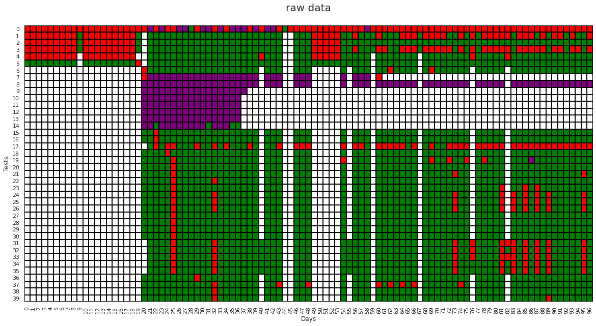
Cells with Purple color in the above graph are the existing flake labels for individual test runs provided by the underlying CI system.

total_existing_flake_label = np.count_nonzero(
    np.array(list(details["values"][:40].values)) == 13
)
print(
    "total number of flakes labeled by the ci system's algorithm:",
    total_existing_flake_label,
)

total number of flakes labeled by the ci system's algorithm: 207

Naive flake method

Below we are annotating a testgrid using the naive flake detection method.

flake_score_threshold = 30
# calculate the flakiness score by naive method for each test in our dataset.
details["naive_flakiness_score"] = details["values"].apply(
    lambda x: naive_flake_calc(x)
)
details["naive_flakiness"] = details.apply(
    lambda x: flake_annotation(
        x["values"], x["naive_flakiness_score"], flake_score_threshold
    ),
    axis=1,
)

plt.figure(figsize=(20, 10))
cmap = colors.ListedColormap(["white", "green", "red", "purple"])
norm = colors.BoundaryNorm(boundaries=[0, 1, 12, 13], ncolors=3)
sns.heatmap(
    np.array(list(details["naive_flakiness"][:40].values)),
    fmt="",
    cmap=cmap,
    norm=norm,
    cbar=False,
    linewidths=0.1,
    linecolor="Black",
)
plt.ylabel("Tests")
plt.xlabel("Days")
plt.title("Naive Method\n", fontsize=20)
plt.show()

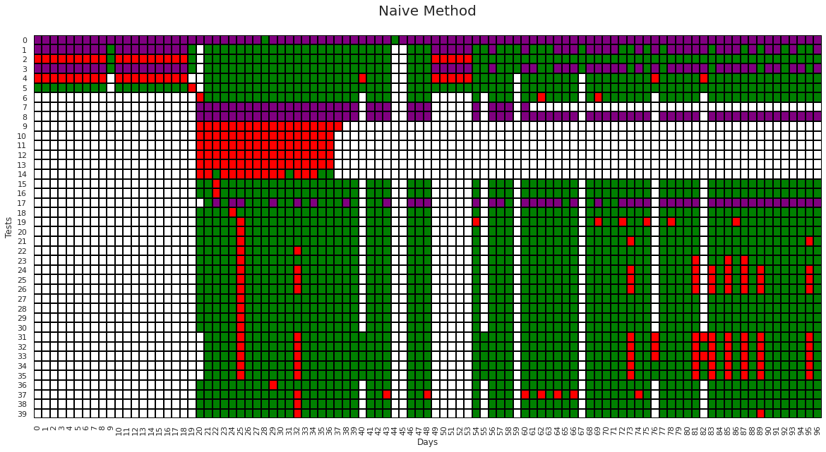
Cells with Purple color in the above graph are the labels given by the naive flake algorithm. We can see the naive flake algorithm is unable to detect many flaky tests such as test number 19, 22, 23, 24, 25, 34, 35, 37. Also, for tests 1, 3 from the time-stamp 0 to 18 consistent failures are occurring, which is not a flake behavior but this method still incorrectly identifies them as flaky.

total_naive_flake_label = np.count_nonzero(
    np.array(list(details["naive_flakiness"][:40].values)) == 13
)
print(
    "Number of flake labels given by the naive flakiness method: ",
    total_naive_flake_label,
)
print(
    "Total flaky tests detected by the `naive flakiness method` is",
    round(total_naive_flake_label / total_existing_flake_label, 2),
    "times \nthe total flaky test detected by the existing testgrid method ",
)

Number of flake labels given by the naive flakiness method:  332
Total flaky tests detected by the `naive flakiness method` is 1.6 times 
the total flaky test detected by the existing testgrid method 

Flip flake method

Below we are annotating testgrid using the flip flake detection method.

flake_score_threshold = 30
## calculate the flakiness score by flip method for each test in our dataset.
details["flip_flakiness_score"] = details["values"].apply(
    lambda x: calc_flakiness_score(x)
)
details["flip_flakiness"] = details.apply(
    lambda x: flake_annotation(
        x["values"], x["flip_flakiness_score"], flake_score_threshold
    ),
    axis=1,
)

plt.figure(figsize=(20, 10))
cmap = colors.ListedColormap(["white", "green", "red", "purple"])
norm = colors.BoundaryNorm(boundaries=[0, 1, 12, 13], ncolors=3)
sns.heatmap(
    np.array(list(details["flip_flakiness"][:40].values)),
    fmt="",
    cmap=cmap,
    norm=norm,
    cbar=False,
    linewidths=0.1,
    linecolor="Black",
)
plt.ylabel("Tests")
plt.xlabel("Days")
plt.title("Flip Flakiness\n", fontsize=20)
plt.show()

Cells with Purple color in the above graph are the labels given by the flip flake algorithm. Though it performed better than naive flake algorithm, but it was still unable to detect flaky behaviors for test number 23 and 24 due to a low occurrence of failures in those tests. Also, for tests 1,2,3,4 from the time-stamp 0 to 18 and for test 17 for time-stamp 74 to 96 consistent failures are occurring, which not a behavior of flaky test but still incorrectly detected as flaky.

total_flip_flake_label = np.count_nonzero(
    np.array(list(details["flip_flakiness"][:40].values)) == 13
)
print(
    "Number of flake labels given by the `flip flakiness` method:",
    total_flip_flake_label,
)
print(
    "Total flaky test detected by the `flip flake` method is",
    round(total_flip_flake_label / total_existing_flake_label, 2),
    "times \nthe total flaky tests detected by the existing testgrid method ",
)

Number of flake labels given by the `flip flakiness` method: 333
Total flaky test detected by the `flip flake` method is 1.61 times 
the total flaky tests detected by the existing testgrid method 

Flip flakiness with optimal distance method

Below we are annotating testgrid using the Flip flakiness with optimal distance method

details["flip_flakiness_optimal"] = details["values"][:40].apply(
    lambda x: calc_optimal_flakiness_score(x, 10)[0]
)

plt.figure(figsize=(20, 10))
cmap = colors.ListedColormap(["white", "green", "red", "purple"])
norm = colors.BoundaryNorm(boundaries=[0, 1, 12, 13], ncolors=3)
sns.heatmap(
    np.array(list(details["flip_flakiness_optimal"][:40].values)),
    fmt="",
    cmap=cmap,
    norm=norm,
    cbar=False,
    linewidths=0.1,
    linecolor="Black",
)
plt.ylabel("Tests")
plt.xlabel("Days")
plt.title("Flip Flakiness with Optimal Distance\n", fontsize=20)
plt.show()

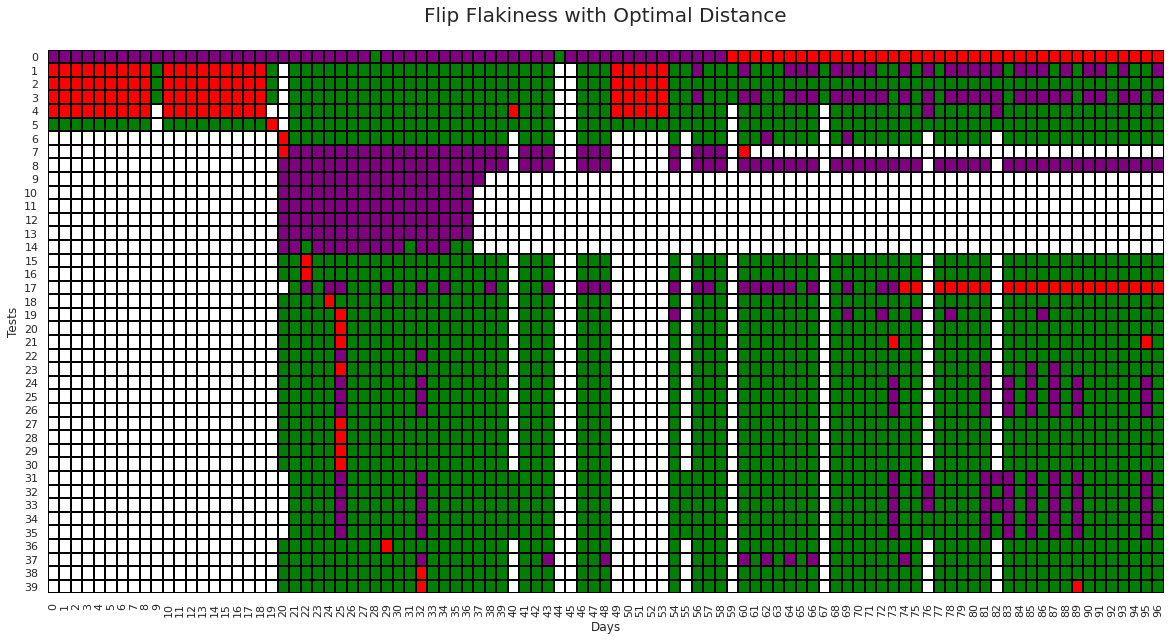
Cells with purple color in the above graph are the labels given by the flip flake with optimal distance algorithm.

In the above figure, we can see that flip flakiness with optimal distance method is able to detect the flaky behavior in test number 4, 19, 22, 23, 24, 25, 34, 35, 37, which naive flake algorithm were failed to detect and test 4 and 23 which flip flake algorithm was failed to detect. Also, it correctly classified flaky tests for test cases 1, 3, 17.

Given the above, its safe to conclude that Flip flakiness with optimal distance works better than naive flakiness and flip flakiness methods on both are example and real world data sets.

total_flip_flake__optimal_label = np.count_nonzero(
    np.array(list(details["flip_flakiness_optimal"][:40].values)) == 13
)
print(
    "Number of flake labels given by the `flip flake optimal distance` method:",
    total_flip_flake__optimal_label,
)
print(
    "Total flaky test detected by the `flip flake optimal distance method` is",
    round(total_flip_flake__optimal_label / total_existing_flake_label, 2),
    "times \nthe total flaky tests detected by the existing testgrid method ",
)

Number of flake labels given by the `flip flake optimal distance` method: 424
Total flaky test detected by the `flip flake optimal distance method` is 2.05 times 
the total flaky tests detected by the existing testgrid method 

Conclusion

TLDR: Flip Flakiness with Optimal Distance is best!

In this notebook, we explored 3 different methods for automatically identifying flaky tests.

1. Naive Flakiness: This was our baseline method to compare the performance of the other two methods. This method simply calculates flakiness as a ratio of failed tests over total tests. As we expected, this method performed the worst and should not be used in the future for flake identification.

2. Flip Flakiness: This method relied on counting the number of edges (flips from pass to fail) for a test. Although it performed much better than the naive method, it fell short for longer test examples with flaky regions in an otherwise stable time-series. Moving forward, this method should not be used either.

3. Flip Flakiness with Optimal Distance: This method extended the flip flakiness method by identifying irregular subsets within a test. This was the best performing method explored in this notebook and should be carried forward into the failure type classification tool and serve as the new baseline.

Next Steps

• The current upstream testgrid repo uses both Naive flakiness and Flip flakiness methods for detecting flakes. We should open an issue and suggest including Flip flakiness with optimal distance into their workflow to further improve flake identification.

• One limitation of the work in this notebook is that we only used the results of previous runs as our data to detect flaky tests. This is not the only data available to us. Next, we can try incorporating additional metadata (like git revisions or linked bugzillas) to improve upon our existing flake identification methods. See this article for possible avenues of future development.